🔭 Anomaly Detection in Gaia Data

Summary

Undergraduate research project cross-matching high-precision Gaia astrometry (GCNS) with high-resolution spectroscopy (GALAH DR4) to find and characterize anomalous stars in the solar neighborhood — via t-SNE over physico-chemical parameters (Stage 1, published) and directly over raw spectra (Stage 2, ongoing).

🌌 Overview

My undergraduate research project looks for and characterizes anomalous stars in the solar neighborhood, cross-matching high-precision astrometry from the Gaia Catalogue of Nearby Stars (GCNS) with high-resolution spectroscopy from GALAH DR4. The project is advised by Prof. Dr. Maria Luiza Linhares Dantas (Instituto de Astrofísica, Pontificia Universidad Católica de Chile), with support from CNPq and IFF.

The work is split into two stages, one already published and one ongoing:

1. Unsupervised t-SNE mapping over physico-chemical parameters (completed, published) — reduces the dimensionality of temperature, gravity, metallicity, and kinematics for ~6,000 stars to find clusters and outliers, validating the method with quantitative metrics and characterizing the sample with classic astrophysical diagrams.
2. Anomaly detection directly on raw spectra (ongoing) — replicating Traven et al.’s (2017) methodology for GALAH, applying t-SNE, UMAP, HDBSCAN, Isolation Forest, and autoencoders directly to the pixels of normalized spectra, without going through the survey pipeline’s already-derived parameters.

Note on this text

This page gathers the current state of the research from my working documentation (methodology, literature review, meeting notes). Stage 1 corresponds to already-published results; Stage 2 is active work, with preliminary results — treat it as such.

---

📊 The data

Catalog	What it provides	Size
GCNS (Gaia Catalogue of Nearby Stars, Gaia DR3)	Very high-precision astrometry and photometry	~330,000 stars within 100 pc of the Sun
GALAH DR4 (Buder et al., 2025)	High-resolution spectra (R≈28,000), up to 30 chemical abundances, atmospheric parameters (Teff, log g, [Fe/H]), ages via PARSEC+COLIBRI isochrones, kinematics (Galpy + McMillan 2017 potential)	~1,017,000 stars
Cross-matched sample (GCNS ∩ GALAH DR4)	Stars with complete astrometry and spectroscopy	~6,000 stars

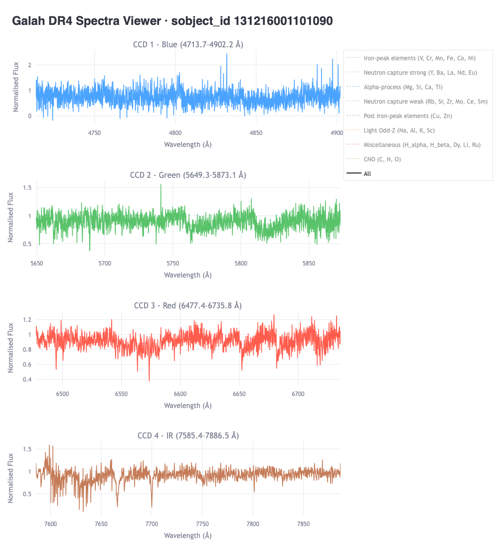
GALAH observes each star in 4 bands (CCDs) of the HERMES spectrograph, at the Anglo-Australian Telescope: blue (4718–4903 Å), green (5649–5873 Å), red (6481–6739 Å), and infrared (7590–7890 Å), each with 4,096 pixels — meaning each spectrum is a 16,384-dimensional vector before any reduction.

The tool I built to explore the spectra

To inspect individual spectra during the analysis, I developed a public web viewer for GALAH DR4 spectra — it shows a star’s 4 bands (by sobject_id), with wavelength regions annotated by chemical element group (iron-peak elements, neutron capture, α-process, CNO, Hα/Hβ, etc.):

---

1️⃣ Stage 1 — t-SNE mapping over physico-chemical parameters (published)

Instead of plotting pre-chosen, hand-picked diagrams, I fed t-SNE directly with each star’s physico-chemical and kinematic parameters (Teff, log g, [Fe/H], [Mg/Fe], and velocity components), letting the algorithm find clusters on its own, only coloring by known parameters afterward as an honesty check on the method.

Quantitative validation — I tested a perplexity grid from 15 to 90 and measured:

• KL divergence — decreases steadily with perplexity.
• Trustworthiness — between ~0.89 and 0.95 (stable).
• Continuity — between ~0.97 and 0.98 (stable).

Both neighborhood-preservation metrics stayed high and stable, indicating the 2D projection preserves both local structure (perplexity 30) and global structure (perplexity 50) of the original high-dimensional space reasonably well. In both, a small standout subgroup appears, with its own internal metallicity gradient — a candidate anomalous population, which motivated Stage 2.

Astrophysical characterization — using the full sample: Kiel diagram (Teff × log g, colored by [Fe/H], with PARSEC+COLIBRI isochrones), Toomre diagram (V × √(U²+W²), separating disk from halo), and Tinsley-Wallerstein diagram ([Mg/Fe] × [Fe/H], separating thin/thick disk). The sample is dominated by F/G/K main-sequence stars, median age ≈ 1.6 Gyr (0.1–14.8 Gyr), median [Fe/H] ≈ −0.19 dex. On the Toomre diagram, 228 stars (3.8% of the sample) have velocity above 100 km/s relative to the Sun — halo-membership candidates, and the most direct kinematic anomaly found so far.

This work was published as:

ANDRADE, P. H. R. et al. Stellar properties and chemical features of the Gaia Catalogue of Nearby Stars observed by GALAH DR4. Boletim da Sociedade Astronômica Brasileira, 2025.

And presented as a poster at SAB 2025, at the 78th Annual SBPC Meeting (2026), and at this National Observatory Winter School (2026) — see Apresentação de Pesquisa (Portuguese) for the full text of that presentation.

---

2️⃣ Stage 2 — Anomalies straight from the spectra (ongoing)

The standout subgroup from Stage 1 raised a question: does that anomaly still show up if I skip the parameters already derived by GALAH’s pipeline — i.e., if I let the algorithm see the raw spectrum directly? That’s the question driving Stage 2, replicating Traven et al.’s (2017) methodology, who used t-SNE over GALAH DR3 spectra to identify 10 morphological categories of peculiar stars.

Catalog columns vs. spectrum pixels

A central methodological decision was understanding the difference between feeding t-SNE catalog columns (already-derived parameters, as in Stage 1) versus the raw spectrum pixels:

• Catalog columns (e.g., [Fe/H], [Mg/Fe] + orbital actions $J_x$, $J_y$ — an approach also used by da Silva & Smiljanic 2023): low computational cost, direct interpretation, but the clustering becomes dependent on the models that generated those columns — a systematic pipeline error (e.g., a poorly-fit log g for a cool star) contaminates the clustering.
• Spectrum pixels (the normalized flux vector, raw data): clusters by morphological similarity of the light itself, immune to stellar atmosphere model errors — better for finding uncataloged binaries or instrument defects, but computationally more expensive and without a ready “physical label” (each cluster’s cause must be inspected manually).

What’s already been tested

I ran t-SNE over the normalized spectra (HDU 1 of each star/CCD’s FITS file) under several configurations, comparing against the column-based approach:

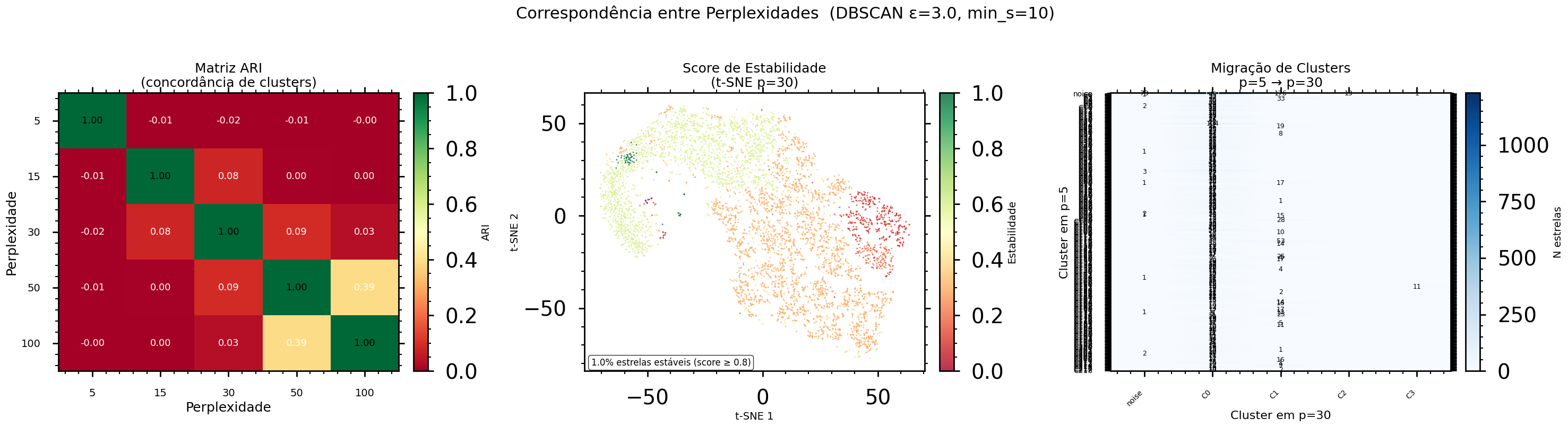
I also quantitatively tested cluster stability across different perplexities, using the Adjusted Rand Index (ARI) to measure agreement between clusters obtained at each perplexity, and tracking how individual stars “migrate” between clusters as this hyperparameter varies:

Comparing dimensionality-reduction + clustering techniques

I tested three combinations of dimensionality reduction + clustering over the spectra, with preliminary results:

Combination	Observed result
UMAP + HDBSCAN	Best balance so far: 6 clusters, few outliers (~25)
t-SNE + DBSCAN	More granular, but initially over-segmented (86+ clusters); improved by tuning ε
PCA + HDBSCAN	Many outliers (~4,469) — evidence that spectral structure is nonlinear and PCA doesn’t capture it well

I also tested two anomaly detectors directly on the embedding: Isolation Forest (assumed 10% contamination, inspired by the fraction of peculiar spectra found by Traven et al. 2017) and a simple autoencoder (MLPRegressor, 4096→64 encoder, threshold at the 95th percentile of reconstruction error) — both still in cross-validation against Traven et al.’s (2017) morphological categories.

---

🗓️ Discussions and decisions (timeline)

Summary of the main methodological decisions made throughout the project, from meeting notes:

• 2026-03-29 — Sample definition (GCNS 330k, GALAH AllStars 980k, cross-matched sample 6k, spectra 24k) and first t-SNE tests on raw spectra, with CCD-inconsistency issues for the same star.
• 2026-03-30 — Cleaning spurious data (negative Teff/log g), standardization of spectrum vectors before t-SNE.
• 2026-04-11 — Cross-review of reference papers (GALAH DR4, Traven et al. 2017) to decide between using raw CCDs or the derived catalog (AllSpec).
• 2026-05-04 — Discussion on the difference between feeding t-SNE catalog columns vs. spectrum pixels (see section above); building and publishing the spectrum viewer; preliminary classification of stars by spectral type (OBAFGKM) from Teff.

---

🚧 Next steps

• Validate the clusters found in Stage 2 with HDBSCAN over the t-SNE projection, comparing directly against Traven et al.’s (2017) 10 morphological categories.
• Cross-match Stage 2’s spectral outliers with the kinematic/chemical subgroup found in Stage 1, to check whether they’re the same population.
• Systematically compare Isolation Forest, autoencoder, and HDBSCAN as anomaly detectors, with precision/recall metrics against known labels.
• Add more chemical tagging diagnostics to test whether the anomalous group is in fact a separate chemical population.

---

📚 Main bibliography

• Traven et al. (2017) — The GALAH survey: classification and diagnostics with t-SNE reduction of spectral information — base methodology for Stage 2.
• Buder et al. (2025) — GALAH DR4.
• Gaia Collaboration et al. (2021) — Gaia Catalogue of Nearby Stars.
• da Silva & Smiljanic (2023) — t-SNE in chemodynamical space (basis for the columns-vs-pixels comparison).
• Hughes et al. (2022) — discovery of extremely metal-poor stars in GALAH DR3 via supervised ML.
• Pettee et al. (2023) — weakly-supervised detection of stellar streams in Gaia (CWoLa).
• See Articles (Portuguese) for the complete reading notes on every paper used in this research.

---

🔗 References and related

• Apresentação de Pesquisa — preparation text for presenting Stage 1 (Portuguese; SBPC 2026 Banner and this Winter School’s Banner).